Intro
For a couple of years, I've been doing research in the field of psychooncology, which basically is “concerned both with the effects of cancer on a person's psychological health as well as the social and behavioral factors that may affect the disease process of cancer and/or the remission of it.” The most influential psycho-oncological journal is named “Psycho-Oncology”. The journal was founded in 1992 and is published monthly by Wiley-Blackwell.
Data
In this blog post, I'll play arround with some bibliographic data from the PubMed data base. With the following query, we receive bibliographical information for every paper published in Psycho-Oncology from 1997 up today.
("Psycho-oncology"[Jour])
As the following screen shot shows, our search query returned 2785 entries. The search results can be downloaded and saved into a .csv file by clicking on the arrow right beside Send to, choosing destination (File) and format (CSV).
Fig. 1: Screenshot from PubMed

R packages
The following code will install load and / or install the R packages required for this blog post.
if (!require("pacman")) install.packages("pacman")
pacman::p_load(pacman::p_load(readr, stringr, ggplot2, qdap, qdapRegex))
Import
The data can be easily imported into R using the read_csv() function from the readr package.
# import .csv file
mydata <- read_csv("pubmed_result.csv")
Data manipulation
With the next code snippet, we do some data manipulation in order to make our data frame tidy. We start with removing the last row of the data frame containing data about a paper published in 1995, remove superfluous headlines, entries without author and select the variables we need for analysis. The str_detect() function stems from the stringr package.
# remove only article from 1995
mydata <- mydata[1:nrow(mydata)-1,]
# remove headlines
mydata <- subset(mydata, str_detect(URL, 'URL')==FALSE)
# remove entries without author
mydata <- subset(mydata, str_detect(Description, 'Author A.')==FALSE)
mydata <- subset(mydata, str_detect(Description, '\\[No authors listed\\]')==FALSE)
# Select variables
mydata <- mydata[, c('Title', 'Description', 'ShortDetails')]
In the next step, we extract the year of publication from the ShortDetails variable. Based on the year variable, we create a variable named time merging the years to four periods of time (five years sub-periods between 1998 and 2016). Furthermore, we calculate the number of authors for each paper using the str_count function of the stringr package. Since each author except for the last is followed by a comma, we just need to count the number of commas and add 1.
# Return Year of publication
mydata$Year <- as.numeric(str_sub(mydata$ShortDetails,
                                  nchar(mydata$ShortDetails)-3,
                                  nchar(mydata$ShortDetails)))
mydata$ShortDetails <- NULL
colnames(mydata) <- c('title', 'authors', 'year')
mydata$time <- ifelse(mydata$year <= 2001, 1,
                      ifelse(mydata$year >= 2002 & mydata$year <=2006, 2,
                             ifelse(mydata$year >= 2007 & mydata$year <=2011, 3, 4)))
mydata$year <- as.factor(mydata$year)
# Categorize years
mydata$time <- factor(mydata$time, levels = c(1:4),
                      labels = c('1997-2001', '2002-2006', '2007-2011', '2012-2016'))
# Calculate number of authors
mydata$auth.n <- str_count(mydata$authors, '\\,') + 1
Before we can plot these data, we need to create 4 more data frames:
df.pupcontaining the number of papers published each year between 1997 and 2006,df.auth.1containing the mean number of authors per paper and year,df.auth.2containing the mean number of authors per paper and time period,df.auth.3containing the maximum number of authors per paper and year,
df.pup <- data.frame(table(mydata$year))
df.auth.1 <- data.frame(aggregate(mydata$auth.n, list(time = mydata$year), mean))
df.auth.2 <- data.frame(aggregate(mydata$auth.n, list(time = mydata$time), mean))
df.auth.3 <- data.frame(aggregate(mydata$auth.n, list(time = mydata$year), max))
Now, we can plot the data using the ggplot2 package.
ggplot(df.pup, aes(x=Var1, y=Freq, fill=0-Freq)) +
  geom_bar(stat="identity", position="dodge", width = .5) +
  geom_text(aes(label=Freq), size = 4,
            fontface=2, hjust =  .45, vjust = -0.75) +
  theme_grey() +
  scale_size_area() +
  scale_y_continuous('', limits=c(0, max(df.pup$Freq)+10), breaks = seq(0, max(df.pup$Freq)+10, by=20)) +
  scale_x_discrete('') +
  theme(legend.position="none") +
  labs(title = "Fig. 2: Number of papers published each year",
       caption = "Data source: PubMed")

Except for a few years, there has been a continuous rise in the number of publications. Since January 2013, Psycho-Oncology has been available exclusively online. Thus, the number of annual papers published is not restricted by requirements of the printed version anymore. Consequently, there was an enormous rise in the number of publications in 2013. However, in the following year (2014) the number of publications declined quite remarkably. The reason for this decline may be a lack of submissions.
ggplot(df.auth.1, aes(x=time, y=x, fill=0-x)) +
  geom_bar(stat="identity", position="dodge", width = .5) +
  geom_text(aes(label=round(x,1)), size = 4,
            fontface=2, hjust =  .45, vjust = -0.75) +
  theme_grey() +
  scale_size_area() +
  scale_y_continuous('', limits=c(0, 10), breaks = seq(0,10, by=2)) +
  scale_x_discrete('') +
  theme(legend.position="none") +
  labs(title = "Fig. 3: Mean number of authors per paper and year",
       caption = "Data source: PubMed")
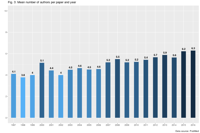
According to figure 3 and 4, the number of authorships per article has been rising over the whole time period. This is in accordance with the general trend towards a rise in the number of personal authors per citation.
ggplot(df.auth.2, aes(x=time, y=x, fill=0-x)) +
  geom_bar(stat="identity", position="dodge", width = .5) +
  geom_text(aes(label=round(x,1)), size = 4,
            fontface=2, hjust =  .45, vjust = -0.75) +
  theme_grey() +
  scale_size_area() +
  scale_y_continuous('', limits=c(0, 10), breaks = seq(0,10, by=2)) +
  scale_x_discrete('') +
  theme(legend.position="none") +
  labs(title = "Fig. 4: Mean number of authors per paper and time period",
       caption = "Data source: PubMed")

Between 1997 and 2016, the mean number of authors per publication has increased from about four to six. The enormous rise in the maximum number of authors (see Fig. 5) supports the idea of an inflation in the number of authors per paper.
ggplot(df.auth.3, aes(x=time, y=x, fill=0-x)) +
  geom_bar(stat="identity", position="dodge", width = .5) +
  geom_text(aes(label=round(x,1)), size = 4,
            fontface=2, hjust =  .45, vjust = -0.75) +
  theme_grey() +
  scale_size_area() +
  scale_y_continuous('', limits=c(0, max(df.auth.3$x)+5), breaks = seq(0, max(df.auth.3$x)+5, by=5)) +
  scale_x_discrete('') +
  theme(legend.position="none") +
  labs(title = "Fig. 5: Max number of authors per paper and year",
      caption = "Data source: PubMed")

Text mining
Before we analyze the data, some janitorial work needs to be done.
We start with (1) defining a list of stopwords, (2, 3) remove non-word characters, (4, 5) replace spaces in two word groups we want to be grouped together, and (6) remove the defined stopwords from the variable containing the citation titles.
sw <- c(Top200Words, 'among') # qdap
mydata$txt <- rm_non_words(mydata$title) # qdapRegex
mydata$txt <- str_replace_all(mydata$txt, "'", "") # stringr
keeps <- c('quality of life', 'health related')
mydata$txt <- space_fill(mydata$txt, keeps, sep = "~~") # qdap
mydata$txt <- rm_stop(mydata$txt, sw,
                      separate = FALSE) # qdap
In the next step, we generate a distribution table for all words of the citation titles. The resulting data frame (df.words) consits of three variables: interval (citation title terms), freq (term frequency), and percent (percentage of the term).
df.words <- dist_tab(breaker(mydata$txt)) # qdap
df.words <- df.words[,c(1, 2, 4)]
df.words <- subset(df.words, percent > 0.5)
df.words <- df.words[order(df.words$percent),]
df.words$interval <- factor(df.words$interval,
                            levels=df.words$interval,
                            labels=df.words$interval,
                            ordered=TRUE)
kable(head(df.words))
| interval | freq | percent | |
|---|---|---|---|
| 666 | coping | 141 | 0.51 |
| 2407 | prostate | 140 | 0.51 |
| 789 | depression | 143 | 0.52 |
| 1335 | health | 147 | 0.53 |
| 2678 | review | 150 | 0.54 |
| 2190 | patient | 154 | 0.56 |
With the next R code we create a list l.txt_time containing four sub lists.
# group titles by time period
l.txt_time <- by(mydata$txt, mydata$time, breaker)
str(l.txt_time)
## List of 4
##  $ 1997-2001: chr [1:2160] "relationship" "between" "trait" "anxiety" ...
##  $ 2002-2006: chr [1:3608] "measurement" "coping" "stress" "responses" ...
##  $ 2007-2011: chr [1:7310] "novel" "stop" "multidisciplinary" "clinic" ...
##  $ 2012-2016: chr [1:14606] "relationship" "between" "objectively" "measured" ...
##  - attr(*, "dim")= int 4
##  - attr(*, "dimnames")=List of 1
##   ..$ mydata$time: chr [1:4] "1997-2001" "2002-2006" "2007-2011" "2012-2016"
##  - attr(*, "call")= language by.default(data = mydata$txt, INDICES = mydata$time, FUN = breaker)
##  - attr(*, "class")= chr "by"
The following code snippet is to convert these four lists into separate data frames, each containing the most frequent citation title terms of the different periods of time.
# time span 1997-2001
df.t1 <- dist_tab(l.txt_time[[1]])
df.t1 <- df.t1[,c(1, 2, 4)]
df.t1 <- subset(df.t1, percent > 0.2)
df.t1 <- df.t1[order(df.t1$percent),]
df.t1$interval <- factor(df.t1$interval,
                         levels=df.t1$interval,
                         labels=df.t1$interval,
                         ordered=TRUE)
df.t1$year <- levels(mydata$time)[1]
# time span 2002-2006
df.t2 <- dist_tab(l.txt_time[[2]])
df.t2 <- df.t2[,c(1, 2, 4)]
df.t2 <- subset(df.t2, percent > 0.2)
df.t2 <- df.t2[order(df.t2$percent),]
df.t2$interval <- factor(df.t2$interval, levels=df.t2$interval,
                         labels=df.t2$interval, ordered=TRUE)
df.t2$year <- levels(mydata$time)[2]
# time span 2007-2011
df.t3 <- dist_tab(l.txt_time[[3]])
df.t3 <- df.t3[,c(1, 2, 4)]
df.t3 <- subset(df.t3, percent > 0.3)
df.t3 <- df.t3[order(df.t3$percent),]
df.t3$interval <- factor(df.t3$interval, levels=df.t3$interval,
                         labels=df.t3$interval, ordered=TRUE)
df.t3$year <- levels(mydata$time)[3]
# time span 2002-2016
df.t4 <- dist_tab(l.txt_time[[4]])
df.t4 <- df.t4[,c(1, 2, 4)]
df.t4 <- subset(df.t4, percent > 0.3)
df.t4 <- df.t4[order(df.t4$percent),]
df.t4$interval <- factor(df.t4$interval, levels=df.t4$interval,
                         labels=df.t4$interval, ordered=TRUE)
df.t4$year <- levels(mydata$time)[4]
Eventually, we create a data frame (df.time) containing the same variables as the data frame df.words and a variable (year) defining the period of time the paper was published.
# merging
df.time <- rbind(df.t1, df.t2, df.t3, df.t4)
df.time <- merge(df.time, df.words, by='interval')
df.time <- df.time[,1:4]
colnames(df.time) <- c('term', 'freq', 'percent', 'year')
df.time$year <- as.factor(df.time$year)
Finally, we plot the most frequent citation title terms over four periods of time.
ggplot(df.time, aes(x=term, y=percent, fill=year)) +
  geom_bar(stat="identity", position="dodge", width = .5) +
  geom_text(aes(label=round(percent,1)), size = 4,
            fontface=2, hjust =  -0.3, vjust = 0.4) +
  theme_grey() +
  scale_size_area() +
  scale_y_continuous('',
                     limits=c(0, max(df.time$percent)+1),
                     breaks = seq(0, max(df.time$percent)+1, by=2)) +
  scale_x_discrete('') +
  theme(legend.position="none") +
  coord_flip() +
  facet_grid(. ~ year) +
  labs(title = "Fig. 6: Most frequent terms in time",
       caption = "Data source: PubMed")

Above all, the terms survivors and distress were increasingly used over time which reflects a growing interest in so-called psychological distress (for a critical discussion see) and cancer survivorship.
